Understand Transformers through Tensor Shapes
Philosophy: dimensions help tell the story. If we understand the tensor shapes, we understand the data flow; and if we understand the data flow, we understand the architecture. If we can trace the journey of an input vector from $d_\text{model} \rightarrow d_\text{head} \rightarrow d_\text{model}$ for example, then we have a good grasp of the transformer.
📒 Link to Google Colab notebook here.
Project features
- Step-by-step analysis of a decoder-only transformer that emphasizes dimensions of key tensors and tie-ins to the big picture, to provide deeper understanding through implementation.
- A built-from-scratch GPT-2 based on ARENA's code, with a clean and "overly commented" implementation to walk through details component-by-component.
Prerequisites: I'm assuming reader comfort with Python, machine learning and neural networks, and matrix multiplication, as well as some familiarity with PyTorch and transformer basics.
How to use this notebook
- To get a unique high-level perspective, read "Overview: GPT-2 Architecture," specifically the subsection "Attention: a Tensor Shapes View."
- For a computation refresher/reference (particularly with
einopscalculations), skip to "Code: GPT-2 Implementation," and refer to specific code snippets/comments. - For a full tutorial, read this document in order: get the high level overview of the architecture, and then go through the code.
This notebook started from my personal notes while self-studying ARENA's AI Safety Curriculum, specifically the Transformer from Scratch chapter (which I highly recommend). I wanted to create a rigorous reference for myself and I hope this is helpful for others as well.
-- Written by LP, updated Jan 2026

(Thanks Dall-E)
Overview: GPT-2 Architecture
Master Blueprint
This is what we'll implement from scratch in the code below!
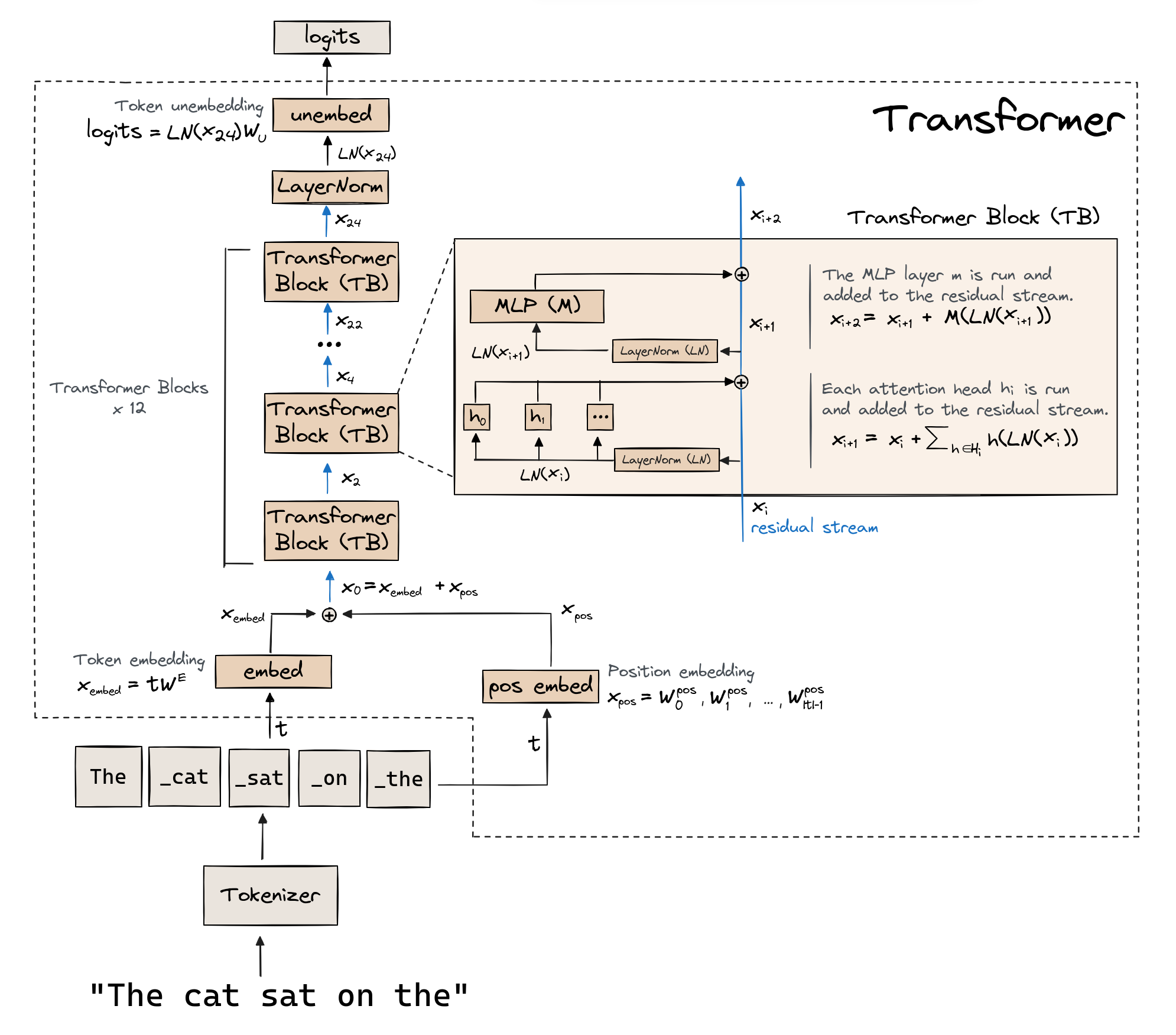
Image from ARENA's Transformer from Scratch notebook
Transformers in a Nutshell
The residual stream
- The residual stream is the shared memory flowing through each layer of the transformer.
- The embedded input is the first state of the residual stream. Each layer in the transformer (either an attention layer or multi-layer perceptron) reads from the stream by taking a copy of the stream as input, and then adds information back into the stream.
Attention layers specialize and move information
- Attention layers are the communication hub for the residual stream.
- Specialization: each attention head reads a copy of the stream and projects it to a lower-dimensional subspace, which forces the head to extract specific features.
- Moving information: each head's attention mechanism "looks" across the entire sequence and copies info from relevant context tokens into each token's representation.
- Writing to memory: these parallel insights are projected and summed simultaneously, and then added to the residual stream.
Multi-layer Perceptron (MLP) layers expand and process information
- Expansion: each layer projects a copy of the residual stream into a higher-dimensional hidden space, which allows the model to map the gathered features to its internal knowledge.
- Process: each layer "thinks" by performing complex non-linear computations (like activations).
- Writing to memory: the result is compressed back to the residual stream dimension and then added to the residual stream.
⏩ Attention: a Tensor Shapes View
About this section
- This section goes through the critical computations used in multi-head self-attention, with a focus on tensor shapes to understand the journey of the input.
- This section parallels the implementation in the Multi-Head Self Attention code section in our
Attentionmodule. - Note that other than batch size and sequence length, axis order can differ in the code implementation compared to the figures.
Q, K, V Matrices
- For each head, project input from embedding space to lower-dimensional "head space" (representation subspace).
- Below we show the computation for Q -- the computations for K, V are analogous.
- $x$ is the input (the normalized residual).

Attention Scores/Weights
High level insight
- For each head, compress the representation subspace into a single scalar value.
- For a given sequence in the batch and given attention head, the attention score between token $i$ and $j$ determines how much information from token $j$ (the source/key) should be moved into the representation of token $i$ (the destination/query).
Technical details
- When we "match indices," we preserve them as a parallel dimension -- for example, here we parallelize over the batch dimension and over each attention head.
- When we sum over an axis (or axes), we collapse the axis/axes -- we mix indices and combine information within the axis/axes, compressing the multi-dimensional info into just a scalar.
- Note that query length and key length are the same as sequence length -- we use difference indices for the second axis of Q and the second axis of K: "query position" and "key position" respectively, to reflect their distinct roles in the attention mechanism.
- The actual attention weights (the result of applying causal masking and softmax to the attention scores) have the same shape as the attention scores (causal masking and softmax preserve dimensions).

Context Vector
- We fill each query token's position with a weighted average of values -- the weights are given by the attention scores, and the values are the actual content being gathered.

Attention Output
- Concatenate the outputs of all heads and then project them back into the residual stream dimension -- this projection is a weighted sum that integrates the specialized information from each head into a single update.

Dimensions Cheat Sheet

Notes:
- Attention weights have two sequence length axes, one for the query and another for the key.
Code: GPT-2 Implementation
Annotations and additions to a built-from-scratch transformer based on ARENA's code.
This recreates the decoder-only architecture of GPT-2.
Code Setup
%pip install -U transformer_lens==2.11.0 einops jaxtyping -q

# Common Python utilities
import os
import sys
import math
from collections import defaultdict
from dataclasses import dataclass
from pathlib import Path
from typing import Callable
from rich import print as rprint
from rich.table import Table

# Pytorch & related shenanigans
import einops
import numpy as np
import torch as t
import torch.nn as nn
from torch import Tensor
from torch.utils.data import DataLoader
from jaxtyping import Float, Int

# Let's get that progress bar!
from tqdm.notebook import tqdm

# TransformerLens mechanistic interpretability library
from transformer_lens import HookedTransformer
from transformer_lens.utils import gelu_new, tokenize_and_concatenate

# Hugging Face
import datasets
from transformers.models.gpt2.tokenization_gpt2_fast import GPT2TokenizerFast
# Don't fold layer norm's learned parameters into the subsequent linear layer
#   -- not folding makes it easier to analyze the layer norm activations themselves
# Don't center the unembedding and writing matrix
#   -- not centering keeps the weights as they were trained in the original GPT-2 model
#   -- note that centering is a trick to make the weights more interpretable

reference_gpt2 = HookedTransformer.from_pretrained(
    "gpt2-small",
    fold_ln=False,
    center_unembed=False,
    center_writing_weights=False,
)
Loaded pretrained model gpt2-small into HookedTransformer
Config
⚠️ Vectorization as Parallelization
In implementation, computation is parallelized across all sequences in a batch in one pass by vectorizing operations along the batch size dimension, which we make the leading dimension.
This is very slick, but can make it difficult to match math equations to code.
For example, the well-known dot product attention formula
$$\text{Attention}(Q, K, V) = \frac{\text{softmax}(QK^T)}{\sqrt{d_k}} V$$
assumes that $Q, K, V$ are 2D matrices. (Here, $d_k$ is equal to d_head, our head dimension.)
In code, these matrices are not 2D. In our code, for example (see the Attention module), $Q, K, V$ are actually 4D (batch_size, n_heads, seq_len, d_head). This is why we use einops, which under-the-hood parallelizes this dot product computation for each sequence within the batch and for each attention head.
Sequence Length vs Max Context Length
A note on seq_len vs n_ctx:
seq_len(sequence length) is the actual tokens the model is processing in a given batch.n_ctxis the maximum context length (it is the architectural limit).
But what about padding?
- We can either pad inputs to the longest sequence in the batch or pad to maximum context length.
- Padding to the longest sequence in the batch is efficient and can prevent unnecessary padding.
- Padding to maximum context length makes sense when the training corpus is, say, long blocks of text that are divided into maximum context length chunks.
- Using
seq_lenhandles both cases.
An interesting note... in the case of padding to the longest sequence in the batch, we should make sure that we see training examples with an original length (no padding) equal to maximum context length -- otherwise we will have untrained weights!
- In our
PosEmbedclass below... we haveself.W_posas shape(n_ctx, d_model) - But we only use
self.W_pos[:seq_len]in the forward pass. - So we want some batches to have
seq_lenequal ton_ctxso that we actually train/update all ofself.W_pos.
@dataclass
class Config:

    d_model: int = 768
    """Token embedding dimension."""

    d_vocab: int = 50257
    """Number of tokens in vocabulary."""

    n_ctx: int = 1024
    """Maximum input length in number of tokens."""

    d_head: int = 64
    """Token embedding dimension per attention head.
    d_model = d_head x n_heads"""

    d_mlp: int = 3072
    """Dimension of hidden layer in the MLP block."""

    n_heads: int = 12
    """Number of attention heads."""

    n_layers: int = 12
    """Number of transformer blocks."""

    layer_norm_eps: float = 1e-5
    """Small constant added to prevent division by zero in layer norm."""

    init_std: float = 0.02
    """Standard deviation of normal random variable for initializing weights."""

    debug: bool = False
    """A toggle to help the user (not used explicitly in this section)."""
Embedding
class Embed(nn.Module):
    """
    Convert tokens to embeddings.
    """

    def __init__(self, cfg: Config):
        super().__init__()
        self.cfg = cfg
        self.W_E = nn.Parameter(t.empty((cfg.d_vocab, cfg.d_model)))
        nn.init.normal_(self.W_E, std=self.cfg.init_std)

    def forward(
        self, tokens: Int[Tensor, "batch_size seq_len"]
    ) -> Float[Tensor, "batch_size seq_len d_model"]:

        # This is mathematically equivalent to O x W_E
        #   where O is the one-hot encoded version of the input
        #   --> this is differentiable!
        return self.W_E[tokens]
Layer Normalization
class LayerNorm(nn.Module):
    """
    For each input sequence in the batch, for each token in that
    input sequence, normalize the token across its embedding dimension.

    Features ("hidden units") of a given token all share the same
    normalization terms.

    But each token has token-specific normalization terms.

    Source: https://www.cs.utoronto.ca/~hinton/absps/LayerNormalization.pdf
    """

    def __init__(self, cfg: Config):
        super().__init__()
        self.cfg = cfg
        self.w = nn.Parameter(t.ones(cfg.d_model))
        self.b = nn.Parameter(t.zeros(cfg.d_model))

    def forward(
        self, residual: Float[Tensor, "batch_size seq_len d_model"]
    ) -> Float[Tensor, "batch_size seq_len d_model"]:

        # Both variables are shape (batch_size, seq_len, 1) -- we keepdim for correct broadcasting
        residual_mean = residual.mean(dim=2, keepdim=True)
        residual_stdev = t.sqrt(t.var(residual, dim=2, unbiased=False, keepdim=True) + self.cfg.layer_norm_eps)

        return (residual - residual_mean)/residual_stdev * self.w + self.b
Position Embedding
class PosEmbed(nn.Module):
    """
    Learned positional embedding.
    """

    def __init__(self, cfg: Config):
        super().__init__()
        self.cfg = cfg
        self.W_pos = nn.Parameter(t.empty((cfg.n_ctx, cfg.d_model)))
        nn.init.normal_(self.W_pos, std=self.cfg.init_std)

    def forward(
        self, tokens: Int[Tensor, "batch_size seq_len"]
    ) -> Float[Tensor, "batch_size seq_len d_model"]:

        batch_size, seq_len = tokens.shape

        pos_embed = self.W_pos[:seq_len].unsqueeze(0) # Shape (1, seq_len, d_model)

        # Repeat across the batch_size dimension
        # The same positional embedding is added to each input sequence
        #   in the batch
        return pos_embed.expand(batch_size, seq_len, self.cfg.d_model)
Transformer Block (Decoder)

Image from an article on decoder-only transformers by Cameron Wolfe, link here.
Computation hints
- Attention is across-token -- in the
Attentionmodule below, the attention scores are the result of aneinopsoperation with two sequence length indices in the output (posn_Qandposn_K). - MLP is per-token -- in the
MLPmodule below, botheinopsoperations in the forward pass have one sequence length index in the output (seq_len).
Multi-Head Self-Attention
class Attention(nn.Module):
    """
    Multi-head attention implemented via tensor parallelism.

    Individual heads are handled as a dimension in the QKV tensors --
        we do NOT make new Attention modules for each attention head.

    Source: https://proceedings.neurips.cc/paper_files/paper/2017/file/3f5ee243547dee91fbd053c1c4a845aa-Paper.pdf
    """

    # Type checking: `IGNORE` is a `Tensor`
    # The empty string means it is a scalar
    IGNORE: Float[Tensor, ""]

    def __init__(self, cfg: Config):
        super().__init__()
        self.cfg = cfg

        # Learned QKV projection matrices
        # Shape (n_heads, d_model, d_head) -- these matrices decompose
        #   the model into specialized heads -- they move stuff from
        #   the model dimension to the head dimension
        self.W_Q = nn.Parameter(t.empty((cfg.n_heads, cfg.d_model, cfg.d_head)))
        self.W_K = nn.Parameter(t.empty((cfg.n_heads, cfg.d_model, cfg.d_head)))
        self.W_V = nn.Parameter(t.empty((cfg.n_heads, cfg.d_model, cfg.d_head)))

        # Writing output
        # Note: these are different dimensions than the QKV counterparts
        # The shape of W_O is NOT a typo here! Shape (n_heads, d_head, d_model) --
        #   this matrix reassembles the heads back into the main stream --
        #   it moves stuff from each head's head dimension to the model dimension
        self.W_O = nn.Parameter(t.empty((cfg.n_heads, cfg.d_head, cfg.d_model)))
        self.b_O = nn.Parameter(t.zeros((cfg.d_model)))

        # Learned QKV biases
        self.b_Q = nn.Parameter(t.zeros((cfg.n_heads, cfg.d_head)))
        self.b_K = nn.Parameter(t.zeros((cfg.n_heads, cfg.d_head)))
        self.b_V = nn.Parameter(t.zeros((cfg.n_heads, cfg.d_head)))

        # We want to "break the symmetry" and initialize weights
        #   to different (random) values -- if they all have the
        #   same value, all their gradients will be the same,
        #   and then network cannot learn
        # Note that the biases are initialized to zero -- this is
        #   standard practice
        # Source: https://www.baeldung.com/cs/ml-neural-network-weights
        nn.init.normal_(self.W_Q, std=self.cfg.init_std)
        nn.init.normal_(self.W_K, std=self.cfg.init_std)
        nn.init.normal_(self.W_V, std=self.cfg.init_std)
        nn.init.normal_(self.W_O, std=self.cfg.init_std)

        # Buffers are tensors that are part of the model's state
        #   but NOT updated during backprop
        # We use this as a mask -- we mask attention scores by
        #   setting masked values to -inf so that after softmax,
        #   we still have valid probabilities
        self.register_buffer("IGNORE",
                             t.tensor(float("-inf"), dtype=t.float32, device=device))

    def forward(
        self, normalized_resid_pre: Float[Tensor, "batch_size seq_len d_model"]
    ) -> Float[Tensor, "batch_size seq_len d_model"]:

        # Move from a dense representation (embedding) to a multi-head view
        # Linear projection from d_model to d_head across all heads simultaneously
        # Each head sees a unique low-rank version of the input
        # q, k, v are all shape (batch_size, seq_len, n_heads, d_head)
        qkv_proj_einops_command = "batch seq d_model, n_heads d_model d_head -> batch seq n_heads d_head"
        Q = einops.einsum(normalized_resid_pre, self.W_Q, qkv_proj_einops_command) + self.b_Q
        K = einops.einsum(normalized_resid_pre, self.W_K, qkv_proj_einops_command) + self.b_K
        V = einops.einsum(normalized_resid_pre, self.W_V, qkv_proj_einops_command) + self.b_V

        # Compute the attention scores
        # For each head, in that head's dimension (subspace), take the dot product
        #   of each query and each key and store that pairwise value
        # Note: posn_Q = posn_K = seq_len -- we just use different names/indices so
        #   that einsum does not collapse/reduce them -- since posn_Q and posn_K are
        #   in the einsum output, we get all the pairwise attention scores between
        #   token i in the query and token j in the key
        attn_einops_command = "batch posn_Q n_heads d_head, batch posn_K n_heads d_head -> batch n_heads posn_Q posn_K"
        attn_scores = einops.einsum(Q,
                                    K,
                                    attn_einops_command) # attention scores: raw
        attn_scores_masked = self.apply_causal_mask(attn_scores / self.cfg.d_head**0.5)

        attn_pattern = attn_scores_masked.softmax(-1) # attention pattern/weights: after softmax

        # Fill each query token's position with a weighted average of values,
        #   the attention pattern (query-key match) defines the weights.
        # Can think of this as moving info from source to destination.
        # Context vector (values that are queried and aggregated according to attention scores)
        # Context vector has shape (batch_size, seq_len, n_heads, d_head)
        z_einops_command = "batch n_heads posn_Q posn_K, batch posn_K n_heads d_head -> batch posn_Q n_heads d_head"
        z = einops.einsum(attn_pattern,
                          V,
                          z_einops_command)

        # Calculate output -- project each head's output back to model dimension and
        #   sum the outputs of heads (sum over n_heads and d_head dimension)
        # This gives the concatenated multi-head attention output, with shape (batch_size, seq_len, d_model)
        attn_out_einops_command = "batch posn_Q n_heads d_head, n_heads d_head d_model -> batch posn_Q d_model"
        attn_out = einops.einsum(z,
                                 self.W_O,
                                 attn_out_einops_command) + self.b_O

        # Note that the above just a more elegant version of the following
        #
        # Concatenate heads -- shape (batch_size, seq_len, n_heads * d_head)
        # Flatten W_O to match -- shape (n_heads * d_head, d_model)
        # Project back to residual stream dimension
        #
        # z_concatenated = einops.rearrange(z, "batch posn_Q n_heads d_head -> batch pos_Q (n_heads d_head)")
        # W_O_flattened = einops.rearrange(self.W_O, "n_heads d_head d_model -> (n_heads d_head) d_model")
        # attn_out = z_concatenated @ W_O_flattened

        return attn_out

    def apply_causal_mask(
        self,
        attn_scores: Float[Tensor, "batch_size n_heads posn_Q posn_K"],
    ) -> Float[Tensor, "batch_size n_heads query_pos key_pos"]:
        """
        By causal masking, we mean that we are turning this model into a predictor
            (not just a pattern matcher). Ensures next-token prediction only
            depends on previous tokens.
        """

        # all_ones is shape (posn_Q, posn_K)
        all_ones = t.ones(attn_scores.size(-2),
                          attn_scores.size(-1),
                          device=attn_scores.device)

        # Don't mask the diagonal -- each token is allowed to look at itself
        mask = t.triu(all_ones, diagonal=1).bool()

        # Again, we parallelize the batch_size and n_heads dimension
        # For each batch and head attention head, we set the above-diagonal
        #   part of the attention scores matrix to -inf (so that the transformer
        #   is not allowed to "look ahead" at future tokens)
        attn_scores.masked_fill_(mask, self.IGNORE)

        return attn_scores
Feed Forward Neural Network
Multi-layer perceptron (MLP) or Feed Forward Neural Network (FFNN).
class MLP(nn.Module):
    """
    Standard MLP -- for each token (in each sequence in the batch),
        apply a fully connected layer (expanding the input to the hidden
        dimension d_mlp), GeLU, and then another fully connected layer
        (return the input to the original embedding dimension d_model).

    Remember: the MLP applies to EACH TOKEN INDEPENDENTLY!
        The MLP is a pointwise/position-wise operation.
    """

    def __init__(self, cfg: Config):
        super().__init__()

        self.cfg = cfg

        # Notice the dimensions are transposed for "in" vs "out"
        self.W_in = nn.Parameter(t.empty((cfg.d_model, cfg.d_mlp)))
        self.W_out = nn.Parameter(t.empty((cfg.d_mlp, cfg.d_model)))

        self.b_in = nn.Parameter(t.zeros((cfg.d_mlp)))
        self.b_out = nn.Parameter(t.zeros((cfg.d_model)))

        nn.init.normal_(self.W_in, std=self.cfg.init_std)
        nn.init.normal_(self.W_out, std=self.cfg.init_std)

    def forward(
        self, normalized_resid_mid: Float[Tensor, "batch_size seq_len d_model"]
    ) -> Float[Tensor, "batch_size seq_len d_model"]:

        # Expansion phase
        # Pre-activation fully connected linear layer output with
        #   shape (batch_size, seq_len, d_mlp) -- expanding the feature space to
        #   a larger MLP hidden state
        pre = einops.einsum(normalized_resid_mid,
                            self.W_in,
                            "batch seq d_model, d_model d_mlp -> batch seq d_mlp") + self.b_in

        # Use GPT2's GeLU function
        # Source: https://github.com/TransformerLensOrg/TransformerLens/blob/main/transformer_lens/utils.py
        post = gelu_new(pre)

        # Down-projection phase
        # Another fully connected linear layer output, with
        #   shape (batch_size, seq_len, d_model) -- projecting back to the model dimension
        mlp_out = einops.einsum(post,
                                self.W_out,
                                "batch seq d_mlp, d_mlp d_model -> batch seq d_model") + self.b_out

        return mlp_out
Transformer Block Integration
class TransformerBlock(nn.Module):
    """
    Remember that each sequence is processed in parallel within a batch.

    Computations per input sequence (after tokenization and positional embedding):
    - Normalize each token relative to its own features
    - Get new context computed using attention
    - Apply residual connection: add attention context and original input together
    - Normalize this sum again -- normalize each transformed token relative to its own features
    - Apply MLP to each transformed token
    - Apply residual connection: add MLP output and current residual stream
        (sum of attention context and original input)
    """

    def __init__(self, cfg: Config):
        super().__init__()
        self.cfg = cfg

        self.ln1 = LayerNorm(cfg)
        self.attn = Attention(cfg)
        self.ln2 = LayerNorm(cfg)
        self.mlp = MLP(cfg)

    def forward(
        self, resid_pre: Float[Tensor, "batch_size seq_len d_model"]
    ) -> Float[Tensor, "batch_size seq_len d_model"]:

        # Each tensor here is shape (batch_size, seq_len, d_model)
        resid_mid = self.attn(self.ln1(resid_pre)) + resid_pre
        resid_post = self.mlp(self.ln2(resid_mid)) + resid_mid
        return resid_post
Unembedding
class Unembed(nn.Module):
    """
    Convert next-word predictions from embedding space to vocab space.
    Each token in the vocabulary gets a logit (unnormalized), where larger logit
        values correspond to higher probabilities of that token being the next one.
    """

    def __init__(self, cfg):
        super().__init__()

        self.cfg = cfg
        self.W_U = nn.Parameter(t.empty((cfg.d_model, cfg.d_vocab)))

        # GPT-2 does not have bias for unembedding step
        self.b_U = nn.Parameter(t.zeros((cfg.d_vocab), requires_grad=False))

        nn.init.normal_(self.W_U, std=self.cfg.init_std)

    def forward(
        self, normalized_resid_final: Float[Tensor, "batch_size seq_len d_model"]
    ) -> Float[Tensor, "batch_size seq_len d_vocab"]:
        """
        Compute logits for each token.
        """

        return einops.einsum(normalized_resid_final,
                             self.W_U,
                             "batch_size seq_len d_model, d_model d_vocab -> batch_size seq_len d_vocab") + self.b_U
⚡ Demo Transformer!
class DemoTransformer(nn.Module):
    """
    Putting it all together :)
    """

    def __init__(self, cfg: Config):
        super().__init__()
        self.cfg = cfg

        self.embed = Embed(cfg)
        self.pos_embed = PosEmbed(cfg)

        # A regular list does not work here -- pytorch will not register the layers
        self.blocks = nn.ModuleList([TransformerBlock(cfg) for _ in range(cfg.n_layers)])

        self.ln_final = LayerNorm(cfg)
        self.unembed = Unembed(cfg)

    def forward(
        self, tokens: Int[Tensor, "batch_size seq_len"]
    ) -> Float[Tensor, "batch_size seq_len d_vocab"]:

        # Initialize residual stream with embedding of original input plus position info
        # (batch_size, seq_len) -> (batch_size, seq_len, d_model)
        residual = self.embed(tokens) + self.pos_embed(tokens)

        # For each layer (transformer block), add to the residual stream
        # (batch_size, seq_len, d_model) -> (batch_size, seq_len, d_model)
        for block in self.blocks:
            residual = block(residual)

        # Clean-up: GPT-2 uses a final layer normalization to stabilize
        #   the residual stream before projecting it back to the vocabulary space
        # (batch_size, seq_len, d_model) -> (batch_size, seq_len)
        logits = self.unembed(self.ln_final(residual))

        return logits
Log Probabilities
Formula Derivation
If $Q$ is our model's distribution and $P$ is the true distribution, then the total cross-entropy of $Q$ relative to $P$ is
$$- \sum_{x \in V} \sum_{c \in C} P(x \mid c) \cdot \text{log } Q(x \mid c),$$ where $C$ includes all possible "contexts" (sequences of tokens, say, up to a certain length), $x$ is the "next token," and $V$ is the vocabulary.
To turn this into a training loss function that we use in practice, we assume the distribution of the training data (the empirical distribution) is the true distribution, so that $P(x \mid \text{context})$ is simply $1$ if $x$ is the observed (true) next token in the data after the given context and $0$ otherwise.
Then the formula becomes
$$ -\frac{1}{N} \sum_{c \in \text{training data}} \text{log } Q\left(x^*(\text{c}) \mid \text{c}\right),$$
where $N$ is the total number of tokens in the training set and $x^*(c)$ is the observed (true) next token in the data after the sequence of tokens $c$. This is the average negative log predicted probability!
In practice, we compute the average over a mini-batch instead of the whole training set.
This shows that next-token prediction training is essentially a classification problem! For each sequence of tokens, we are predicting an integer (from $1$ to $\lvert V \rvert$) (corresponding to the token in the vocabulary that is the next token).
The above formulation is not something that is typically written -- it's more common to find simplified notation. But this formulation it makes clear the assumptions we need to use cross entropy loss, and why we use negative log probability of prediction (i.e. negative log likelihood) interchangeably with cross entropy. Many resources treat cross entropy loss as just another "black box" for LLMs, but exploring more detailed notation clarifies the bridge between sequence modeling and classification.
For additional resources: a five minute primer on cross entropy loss by Adian Liusie here and another explanation of the cross entropy and negative log probability equivalence by Sebastian Raschka here.
def get_log_probs(
    logits: Float[Tensor, "batch_size seq_len d_vocab"],
    tokens: Int[Tensor, "batch_size seq_len"]
) -> Float[Tensor, "batch_size seq_len-1"]:
    """
    Negative log probability (negative log likelihood) is equivalent
        to cross entropy (under the assumption that the observed/empirical
        training distribution is the true distribution).

    This function computes the model's estimated/predicted log probability
        for each true next token.
    """

    # Take the log softmax over the vocabulary dimension
    log_probs = logits.log_softmax(dim=-1) # shape (batch_size, seq_len, d_vocab)

    # The input has length seq_len, so we'll do seq_len-1 next-token predictions
    #   to compare the model's predictions of the input to the actual input
    # For the last token in the sequence, there is no "next token",
    #   so don't include the last token
    log_probs_pred = log_probs[:, :-1]

    # These are the true/actual next tokens
    # Note we need to unsqueeze so that the multi-dimensional lookup indexing works
    true_labels = tokens[:, 1:].unsqueeze(-1) # shape (batch_size, seq_len-1, 1)

    # Gather is multi-dimensional lookup
    # For each true/observed token, get the model's estimated/predicted
    #   log probability for that token
    log_probs_for_tokens = log_probs_pred.gather(dim=-1, index=true_labels).squeeze(-1)

    return log_probs_for_tokens
Validation
Let's verify that our demo transformer successfully recreates GPT-2.
# Load our demo transformer and GPT-2 as a reference

device = t.device("mps" if t.backends.mps.is_available() else "cuda" if t.cuda.is_available() else "cpu")

demo = DemoTransformer(Config()).to(device)
demo.load_state_dict(reference_gpt2.state_dict(), strict=False)
demo.eval()

reference_gpt2.eval()

# Don't auto-print the last object
pass
@t.no_grad()
def compare_models(prompt, demo_model, ref_model, steps=20):
    """
    Validates the demo model by comparing its top-1 predictions
    against the reference model step-by-step.
    """

    tokens = ref_model.to_tokens(prompt).to(device)

    # Table header
    print(f"\nComparing models on prompt: '{prompt}' \n")
    print(f"{'Step':<5} | {'Demo Prediction':<20} | {'Reference Prediction':<20} | {'Match?'}")
    print("-" * 65)

    for i in range(steps):

        demo_logits = demo_model(tokens)
        ref_logits, ref_cache = ref_model.run_with_cache(tokens)

        # Very last token's logits
        demo_next = demo_logits[0, -1].argmax(dim=-1)
        ref_next = ref_logits[0, -1].argmax(dim=-1)

        # Decode for display and check match
        demo_str = ref_model.to_string(demo_next)
        ref_str = ref_model.to_string(ref_next)
        match = "✅" if demo_next == ref_next else "❌"

        print(f"{i+1:<5} | {repr(demo_str):<20} | {repr(ref_str):<20} | {match}")

        # Teacher forcing: append the REFERENCE token to the sequence
        # This ensures that even if the demo misses once, we see if it recovers
        tokens = t.cat([tokens, ref_next.unsqueeze(0).unsqueeze(0)], dim=-1)

    # Check total logit divergence is small
    diff = (demo_logits - ref_logits).abs().max().item()
    print(f"\nFinal Max Logit Difference: {diff:.6f}")
compare_models("Large language models are interesting because ", demo, reference_gpt2)
Comparing models on prompt: 'Large language models are interesting because '

Step  | Demo Prediction      | Reference Prediction | Match?
-----------------------------------------------------------------
1     | '\xa0'               | '\xa0'               | ✅
2     | 'they'               | 'they'               | ✅
3     | ' allow'             | ' allow'             | ✅
4     | ' us'                | ' us'                | ✅
5     | ' to'                | ' to'                | ✅
6     | ' explore'           | ' explore'           | ✅
7     | ' the'               | ' the'               | ✅
8     | ' relationship'      | ' relationship'      | ✅
9     | ' between'           | ' between'           | ✅
10    | ' language'          | ' language'          | ✅
11    | ' and'               | ' and'               | ✅
12    | ' cognition'         | ' cognition'         | ✅
13    | '.'                  | '.'                  | ✅
14    | ' '                  | ' '                  | ✅
15    | '\xa0'               | '\xa0'               | ✅
16    | 'In'                 | 'In'                 | ✅
17    | ' this'              | ' this'              | ✅
18    | ' paper'             | ' paper'             | ✅
19    | ','                  | ','                  | ✅
20    | ' we'                | ' we'                | ✅

Final Max Logit Difference: 0.000107
# Greedily generate next tokens with our demo transformer

test_string = "I hope you enjoyed this tutorial. "
test_tokens = reference_gpt2.to_tokens(test_string).to(device)

for _ in range(20):
    with t.no_grad():
        logits = demo(test_tokens)
        next_token = logits[0, -1].argmax(dim=-1).unsqueeze(0).unsqueeze(0)
        test_tokens = t.cat([test_tokens, next_token], dim=-1)

print(f"\nDemo Generation: {reference_gpt2.to_string(test_tokens[0])}")
Demo Generation: <|endoftext|>I hope you enjoyed this tutorial. I hope you enjoyed reading it. I hope you enjoyed reading my blog.